This page contains code that performs gradient descent to solve a simple linear regression problem. The interesting part are the Mean Squared Error (MSE) and log cost of the operations. The first part uses a dataset from Andrew Ng's Machine Learning course. The second part randomly generates a set of points to apply linear regression to then takes different values for \( \alpha \). This was a quick but fun little project! If you're trying to learn about linear regression and gradient descent the best thing to do is play around with the code and make your own version. Have fun!
# Code by Eric Johnson at FocusNumeric.net
import numpy as np
import matplotlib.pyplot as plt
import random

xVec = np.random.rand(100)
a = random.randint(-100,100)
b = random.randint(-100,100)
noise = np.random.normal(loc=np.mean(a),scale=np.log(np.abs(b)),size=len(xVec))

yVec = a*xVec + b + noise

# Plot raw data without regression line
plt.plot(xVec, yVec, 'ro')
plt.title("Before Linear Regression Line")
plt.show()

# initialize vectors
m = len(xVec)
# X has ones in first column to have 'y intercept' term
X = np.asarray([np.ones(m), xVec])
# initialize parameters as (0,0)^T
theta = np.zeros((2, 1))

def computeCost(X, y, theta):
    m = len(y)
    J = 0
    h = np.dot(np.transpose(X), theta)

    residSq = 1 / (2 * m) * np.square(h - y)
    J = np.sum(residSq)
    return J

J = computeCost(X, yVec, theta)

numIt = 10000
alpha = 0.01

def gradientDescent(X, y, xVec, theta, alpha, numIt):
    m = len(y)
    J_Hist = np.zeros((numIt, 1))

    for i in range(0, numIt):
        h = np.dot(np.transpose(theta), X)
        theta1 = theta[0] - alpha * (1 / m) * np.sum(h - y)
        theta2 = theta[1] - alpha * (1 / m) * np.sum(np.multiply((h - y), X[1, :]))
        theta[0] = theta1
        theta[1] = theta2
        J_Hist[i] = computeCost(X, y, theta)

    return J_Hist, theta

J_Hist, theta = gradientDescent(X, yVec, xVec, theta, alpha, numIt)

print(theta[0])
print(theta[1])

# plot results
regLine = theta[1] * xVec + theta[0]
plt.subplot(1,2,1)
plt.plot(xVec, yVec, 'ro')
plt.title("With Linear Regression Line")
plt.plot(xVec, regLine, '-')
plt.subplot(1,2,2)
plt.plot(range(0,len(J_Hist)),np.log(J_Hist))
plt.title("Cost vs. Iterations")
plt.xlabel("Iteration")
plt.ylabel("Cost")
plt.show()
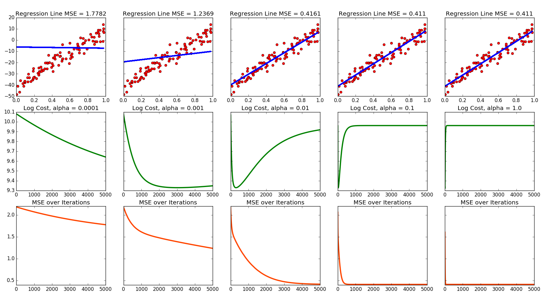
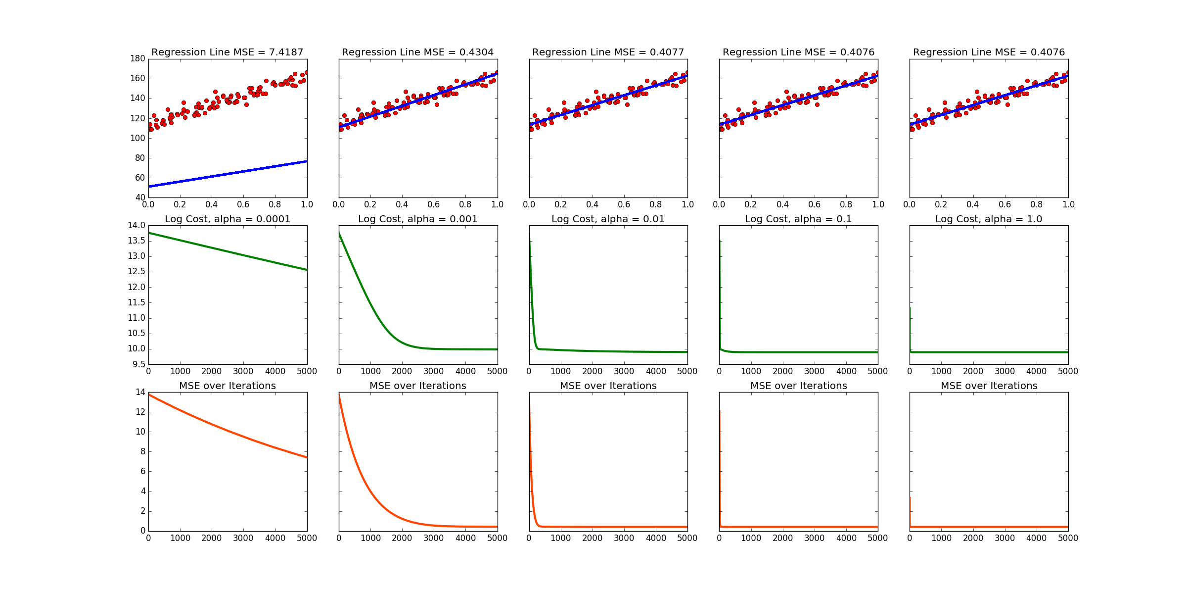
Alright - straighforward enough. But what influence does \( \alpha \) have on picking a regression line and on the cost? That's the question that inspired me to play around with \( \alpha \) and write 'Part II.'
Part II:
I am *always* trying to generalize code to make it reusable. So this generates a random $x$ vector with 100 points. Then it picks two random integers between -100 and 100 to use as slope and y-intercepts. Then Numpy is used to create a little noise and plots the vector
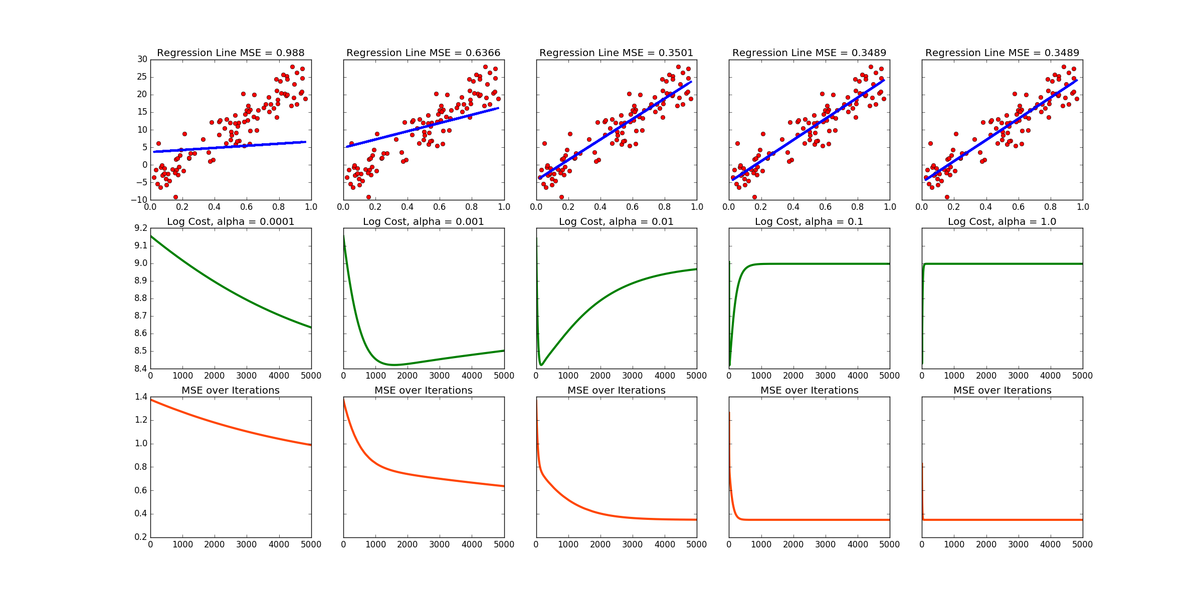
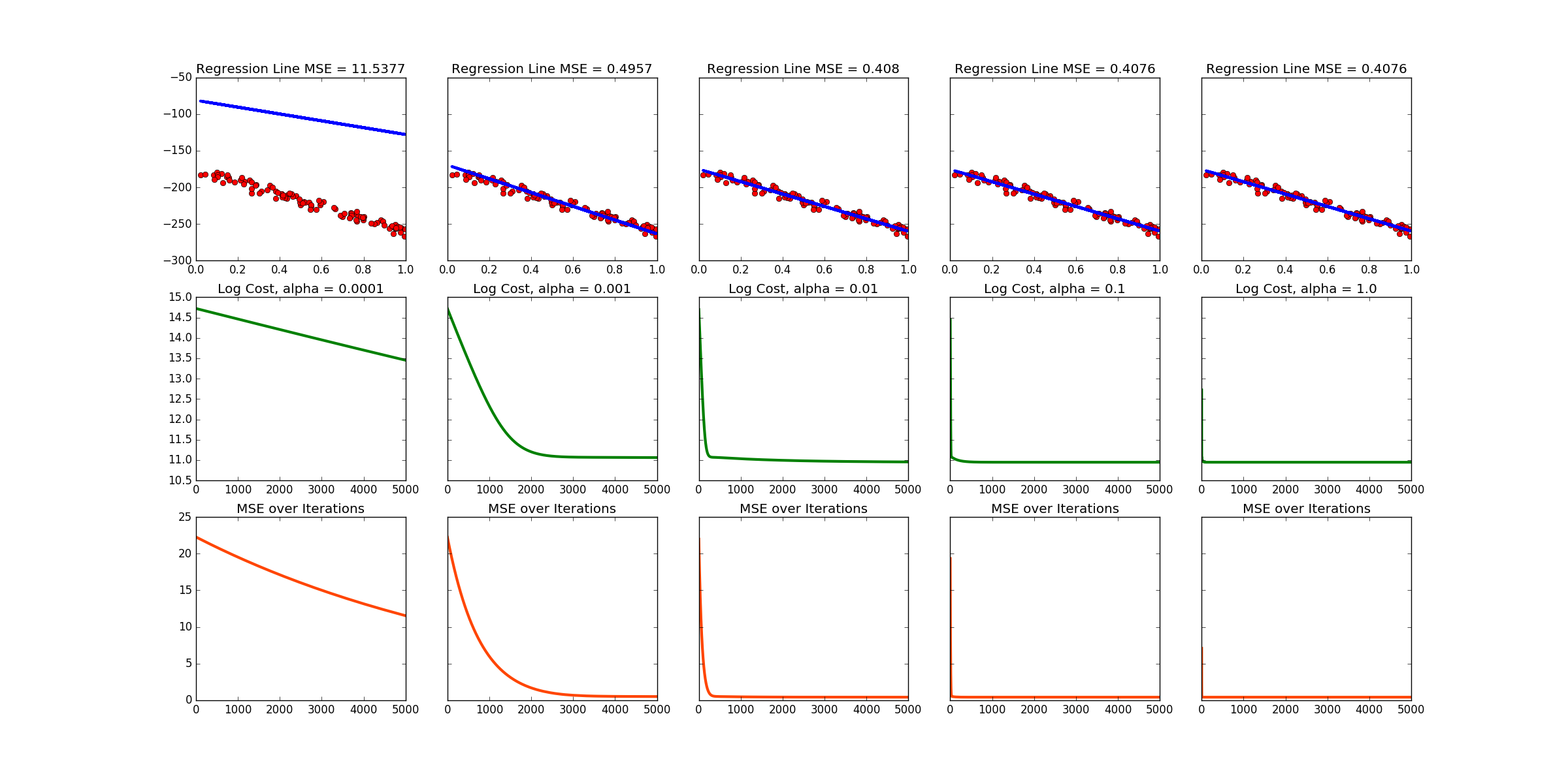
Note that this produces a different data set and line every time the code is run! Below is the output of one run. There are links to more at the bottom of this page.
Future addition: As is, the number of GD iterations is fixed at 5000. But I'd like to do it so that it only does iterations until the difference between costs reaches some threshold value. That would be better. I'll do it later!
# Code by Eric Johnson at FocusNumeric.net

import numpy as np
import matplotlib.pyplot as plt
import random

xVec = np.random.rand(100)
a = random.randint(-100,100)
b = random.randint(-100,100)
noise = np.random.normal(loc=np.mean(a),scale=np.log(np.abs(b)),size=len(xVec))

yVec = a*xVec + b + noise

# Plot raw data without regression line
plt.plot(xVec, yVec, 'ro')
plt.title("Random Data")
plt.show()

# initialize vectors
m = len(xVec)
# X has ones in first column to have 'y intercept' term
X = np.asarray([np.ones(m), xVec])

def computeCost(X, y, theta):
    m = len(y)
    J = 0
    h = np.dot(np.transpose(X), theta)

    residSq = 1 / (2 * m) * np.square(h - y)
    J = np.sum(residSq)
    return J

numIt = 5000

def gradientDescent(X, y, xVec, theta, alpha, numIt):
    m = len(y)
    J_Hist = np.zeros((numIt, 1))
    E_Hist = np.zeros((numIt, 1))

    for i in range(0, numIt):
        h = np.dot(np.transpose(theta), X)
        theta1 = theta[0] - alpha * (1 / m) * np.sum(h - y)
        theta2 = theta[1] - alpha * (1 / m) * np.sum(np.multiply((h - y), X[1, :]))
        theta[0] = theta1
        theta[1] = theta2
        J_Hist[i] = computeCost(X, y, theta)
        intReg = theta[1] * xVec + theta[0]
        E_Hist[i] = calculateError(yVec,intReg)

    return J_Hist, theta, E_Hist

def calculateError(yData,regLine):
    residuals = yData - regLine
    error = np.square(residuals)
    error = np.sum(error)
    error = np.sqrt(error)
    error = error/100
    error = round(error,4)
    return error

alphaList = np.asarray([0.0001,0.001,0.01,0.1,1])
# Note:  alpha = 10 is too large.  Causes memory overflow.

# alpha = alphaList[0]
# initialize parameters as (0,0)^T
theta = np.zeros((2, 1))
J_Hist0, theta0, E_Hist0 = gradientDescent(X, yVec, xVec, theta, alphaList[0], numIt)
regLine0 = theta0[1] * xVec + theta0[0]
error0 = calculateError(yVec,regLine0)

# alpha = alphaList[1]
# initialize parameters as (0,0)^T
theta = np.zeros((2, 1))
J_Hist1, theta1, E_Hist1 = gradientDescent(X, yVec, xVec, theta, alphaList[1], numIt)
regLine1 = theta1[1] * xVec + theta1[0]
error1 = calculateError(yVec,regLine1)

# alpha = alphaList[2]
# initialize parameters as (0,0)^T
theta = np.zeros((2, 1))
J_Hist2, theta2, E_Hist2 = gradientDescent(X, yVec, xVec, theta, alphaList[2], numIt)
regLine2 = theta2[1] * xVec + theta2[0]
error2 = calculateError(yVec,regLine2)

# alpha = alphaList[3]
# initialize parameters as (0,0)^T
theta = np.zeros((2, 1))
J_Hist3, theta3, E_Hist3 = gradientDescent(X, yVec, xVec, theta, alphaList[3], numIt)
regLine3 = theta3[1] * xVec + theta3[0]
error3 = calculateError(yVec,regLine3)

# alpha = alphaList[4]
# initialize parameters as (0,0)^T
theta = np.zeros((2, 1))
J_Hist4, theta4, E_Hist4 = gradientDescent(X, yVec, xVec, theta, alphaList[4], numIt)
regLine4 = theta4[1] * xVec + theta4[0]
error4 = calculateError(yVec,regLine4)

# Plot everything
f, axarr = plt.subplots(3, 5, sharey='row')
axarr[0,0].plot(xVec,yVec,'ro')
axarr[0,0].plot(xVec,regLine0,'-', linewidth = 3)
axarr[0,0].set_title("Regression Line MSE = %s" %(error0))
axarr[1,0].plot(range(0,len(J_Hist0)),np.log(J_Hist0), color = 'g', linewidth = 3)
axarr[1,0].set_title("Log Cost, alpha = 0.0001")
axarr[2,0].plot(range(0,len(E_Hist0)),E_Hist0, color = 'orangered', linewidth = 3)
axarr[2,0].set_title("MSE over Iterations")

axarr[0,1].plot(xVec,yVec,'ro')
axarr[0,1].plot(xVec,regLine1,'-', linewidth = 3)
axarr[0,1].set_title("Regression Line MSE = %s" %(error1))
axarr[1,1].plot(range(0,len(J_Hist1)),np.log(J_Hist1), color = 'g', linewidth = 3)
axarr[1,1].set_title("Log Cost, alpha = 0.001")
axarr[2,1].plot(range(0,len(E_Hist1)),E_Hist1, color = 'orangered', linewidth = 3)
axarr[2,1].set_title("MSE over Iterations")

axarr[0,2].plot(xVec,yVec,'ro')
axarr[0,2].plot(xVec,regLine2,'-', linewidth = 3)
axarr[0,2].set_title("Regression Line MSE = %s" %(error2))
axarr[1,2].plot(range(0,len(J_Hist2)),np.log(J_Hist2), color = 'g', linewidth = 3)
axarr[1,2].set_title("Log Cost, alpha = 0.01")
axarr[2,2].plot(range(0,len(E_Hist2)),E_Hist2, color = 'orangered', linewidth = 3)
axarr[2,2].set_title("MSE over Iterations")

plt.show()
Links to dataset, Python code, and some sample program output
Data from Dr. Ng's ML course.
linearRegression.py
linearRegressionVariedAlpha.py
Sample output no. 1
Sample output no. 2
Sample output no. 3
Sample output no. 4
Sample output no. 5
Sample output no. 6
Sample output no. 7
Sample output no. 8
Sample output no. 9
Sample output no. 10
Depending on your browser you may have to 'save as.'
To execute the Python code just go to the folder containing the .py file and type "python3 linearRegressionVariedAlpha.py" in Bash.
Some places to find out more:
- Yay Numpy!: Numpy