One of the best things about R is how much it has been extended with libraries to perform different tasks. One of my favorite packages is Markdown. With Markdown, R can be used to produce beautiful PDFs, HTML, Microslop Word Docs and more. Even better, LaTeX code can be embedded in these documents so mathematics can be notated correctly. Truly excellent!
I produced code to produce PDF reports for UPS, STS, and PDU data at work. I'd love to post that code because it's 25+ pages of R code that does serious data manipulation, analysis, and plotting. However, I don't own that code - and I certainly do not own the data! Fortunately I have some other data I can use to create a good Markdown example.
I am assuming a few things if you are going to follow along.
- You already have R installed.
- You have some kind of LaTeX system installed.
- ... and both are working!
- You are willing to look up some built-in R functions or LaTeX if you don't understand them.
- I don't explain any of the LaTeX commands. LaTeX is worth learning - but you don't have to know it to follow along.
There are a few things you have to do to run Markdown. Run the following in the R GUI (or R Studio):
install.packages("markdown")
install.packages("xtable")
install.packages("knitr")
library(markdown)
library(xtable)
library(knitr)
sudo apt-get install texlive-fullMarkdown documents are a little different from standard R files. The file extension is *.Rmd rather than *.R, which contains R code, LaTeX (possibly), and formatting information that is interpreted by the Markdown package. A markdown document is 'rendered' rather than executed. Enter something like this in the command line to produce a PDF document:
render("MyMarkdownFile.Rmd", output_format="pdf_document",output_file=paste("MyMarkdownOutputFile", Sys.Date(), ".pdf"))
Of course you can put these in an R function to generate several of these in a batch. For example, "RenderReports.R" which renders four separate PDFs from MyMarkdownFile1.Rmd, MyMarkdownFile2.Rmd, etc.
RenderReports <- function(){
 library(markdown)  # load the required libraries if you haven't done so already.  Doing it twice won't hurt anything.
 library(xtable)
 library(knitr)
 render("MyMarkdownFile1.Rmd", output_format="pdf_document",output_file=paste("MyMarkdownOutputFile1", Sys.Date(), ".pdf"))
 render("MyMarkdownFile2.Rmd", output_format="pdf_document",output_file=paste("MyMarkdownOutputFile2", Sys.Date(), ".pdf"))
 render("MyMarkdownFile3.Rmd", output_format="pdf_document",output_file=paste("MyMarkdownOutputFile3", Sys.Date(), ".pdf"))
 render("MyMarkdownFile4.Rmd", output_format="pdf_document",output_file=paste("MyMarkdownOutputFile4", Sys.Date(), ".pdf"))
 }
source("RenderReports.R")
RenderReports()
I have a nice dataset produced by connecting my oscilloscope to my TENS unit. The data itself is very simple: just one column containing AC voltage. Here is an image of what the data looks like (plotted in Mathematica):
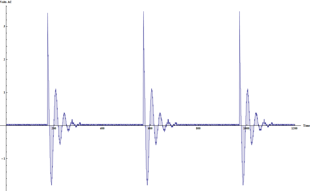
A TENS unit is a medical device that delivers a little pulse of AC voltage to exercise muscles. (I have one because someone ran over me with a car in the parking lot of IBM last year.) It's a nice medication-free way of relieving pain.
There are a few issues with the actual data as I collected it. First, I accidentally set my oscilloscope probes to something other than "1x." A dumb mistake on my part - but to be fair the setting was buried in the oscilloscope settings menu. That means that I have to transform the data so that the voltage output is closer to what my Fluke 87V read. Also, there's no actual "time" data since the oscilloscope didn't produce a time column. We can operate on the data without this... But the TENS unit produces pulses at a measurable frequency and subtle differences in that frequency are noticeable for a user. I'll produce both a meaningful "time" vector for plotting and transform the voltage data here. There are a few things I'd like R to do with the data.
Everything is included in the comments!
# TENS data with R, Markdown and LaTeX... [Focus Numeric](http://focusnumeric.net/)
Note: You call LaTeX by using '\( stuff \)' (inline) and double dollar signs for equation blocks.

```{r echo=TRUE, results='asis'}

# Pull OscData from the dataset
    OscData <- read.csv("OscOutput7.csv")
# Create a plotting vector -- find the length first, then create a plotting sequence
# "plotVec".  I want to start the vector at 0 so we have to adjust the length appropriately.
    dataLength <- length(OscData$VAC.Out)
    plotVec <- 0:(dataLength-1)
# and plot with:
# plot(plotVec,OscData$VAC.Out, type="l", col="blue", main="Raw (unscaled) OscData
# from TENS unit", xlab="Time", ylab="Volts AC")

```
```{r echo=FALSE, results='asis'}

	plot(plotVec,OscData$VAC.Out, type="l", col="blue", main="Raw (unscaled) OscData from TENS unit", xlab="Time", ylab="Volts AC")

```
```{r echo=TRUE, results='asis'}
    k <- 3.457 / 284
	scaledData <- k*OscData$VAC.Out
```
```{r echo=TRUE, results='asis'}
    which(OscData$VAC.Out>275)
```
```{r echo=TRUE, results='asis'}
    timeVec <- 1/20000 * plotVec
```
which gives us fully scaled data.  Here's an updated plot:

```{r echo=FALSE, results='asis'}
	plot(timeVec,scaledData, type="l", col="blue", main="Fully scaled TENS data", xlab="Time", ylab="Volts AC")
```
```{r echo=TRUE, results='hide'}
    which(scaledData==0)
```
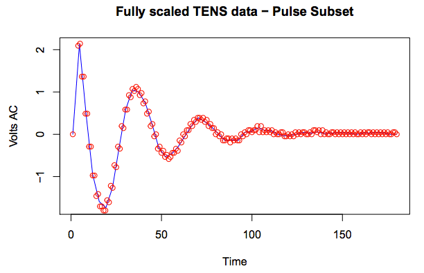
```{r echo=FALSE, results='asis'}
    pulseSubset <- scaledData[171:350]
    plotPulse <- timeVec[171:350]
    plot(approx(pulseSubset), type="l", col="blue", main="Fully scaled TENS data - Pulse Subset", xlab="Time", ylab="Volts AC")
    points(pulseSubset, col="red")
```
That should provide a simple Markdown example that has a little LaTeX mixed in.
Links to TENS data and the actual Markdown file.
Raw oscilloscope output data
TENS.Report.Rmd file
TENS.Report rendered as PDF
Depending on your browser you may have to 'save as.'
Some places to find out more:
- LaTeX installation: Obtaining LaTeX at latex-project.org
- The main Markdown site: R Markdown. The assumption is generally that you will be using R Studio. You can run Markdown in the regular R GUI without any complication. I can't use R Studio at work because of security restrictions but can use Markdown anyway.
- Pandoc is required for running Markdown. See http://pandoc.org/
- A great R resource! See: "R In Action" from Manning.com It is worth a little extra to get the second edition. (Markdown isn't even covered in the first edition.) I highly recommend this book.