Graph Eigenvalues

I wanted to write some simple Mathematica code to produce random graphs and calculate eigenvalues for the adjacency matrices of those graphs.

Adjacency matrices are matrix representations of the connections in a graph. Here is a definition:

Let $ G $ be a graph of order $ n $. Let the vertex set $ V = \{ v_1, v_2, ..., v_n \}. $ An edge set $ E $ contains pairs $ ij = ji $ where there is an edge between vertices $ v_i $ and $ v_j $. The Adjacency matrix $ A = a_{ij} $ is defined by: $$ a_{ij} = \begin{cases} 1 &\text{if }ij \text{ is an edge } \\ 0 &\text{ otherwise} \end{cases} $$

Graphs may be reflexive or irreflexive. A vertex in an irreflexive graph may not connect to itself via an edge. A reflexive graph may contain vertices that are connected to themselves via an edge. If a graph is irreflexive all diagonal matrix entries are 0. A reflexive graph may have 1's on the diagonal where vertices are connected to themselves by an edge. The matrix $ A $ is symmetric and all nonzero entries are positive.

Graphs may also be directed or undirected. The edge in an undirected graph is nondirectional. In other words, if there's an edge between two vertices $ v_1 $ and $ v_2 $, then $ v_1 $ is connected to $ v_2 $ and $ v_2 $ is connected to $ v_1 $. However, in a directed graph, $ v_1 $ may be connected to $ v_2 $ with an edge - but that doesn't mean $ v_2 $ is necessarily connected to $ v_1 $. The adjacency matrix naturally changes with these cases. The graph here may not be symmetric.

Fortunately the ordering of the vertices does not matter when constructing an adjacency matrix. Suppose we have two different spellings, say $ E $ and $ E' $ and $ V $ and $ V' $ for the vertex and edge set of otherwise identical graphs $ G $ and $ G'$. Suppose $ A $ and $ A' $ are the adjacency matrices of graphs $ G $ and $ G' $. Then $ A' $ is simply a permutation matrix $ P^{-1} A P $ of $ A$. The eigenvalues of of these similar matrices are equal.

Here is a simple example to illustrate that point. Consider graphs $ G_1 $ and $ G_2 $.

Graph $ G_1 $: GraphG1 , with adjacency matrix: $ A_1 = \begin{pmatrix} 0 & 0 & 1 & 0 & 1 \\ 0 & 0 & 1 & 0 & 0 \\ 1 & 1 & 0 & 1 & 1 \\ 0 & 0 & 1 & 0 & 0 \\ 1 & 0 & 1 & 0 & 0 \end{pmatrix}$ and eigenvalues / eigenvectors (computed in R)

> A1 <- matrix(c(0,0,1,0,1,0,0,1,0,0,1,1,0,1,1,0,0,1,0,0,1,0,1,0,0),5,5 )
> eigen(A1, symmetric=TRUE)
$values
[1]  2.342923e+00  4.706834e-01  1.110223e-16 -1.000000e+00 -1.813607e+00

$vectors
           [,1]       [,2]          [,3]          [,4]       [,5]
[1,] -0.4734862 -0.4559848  0.000000e+00  7.071068e-01  0.2605546
[2,] -0.2713941  0.5127870 -7.071068e-01 -2.220446e-16  0.4042212
[3,] -0.6358555  0.2413603  1.110223e-16 -4.440892e-16 -0.7330982
[4,] -0.2713941  0.5127870  7.071068e-01 -2.775558e-16  0.4042212
[5,] -0.4734862 -0.4559848  1.110223e-16 -7.071068e-01  0.2605546

Graph $ G_2 $: GraphG2 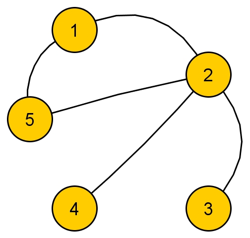, with adjacency matrix: $ A_2 = \begin{pmatrix} 0 & 1 & 0 & 0 & 1 \\ 1 & 0 & 1 & 1 & 1 \\ 0 & 1 & 0 & 0 & 0 \\ 0 & 1 & 0 & 0 & 0 \\ 1 & 1 & 0 & 0 & 0 \end{pmatrix}$ and eigenvalues / eigenvectors (computed in R)

> A2 <- matrix(c(0,1,0,0,1,1,0,1,1,1,0,1,0,0,0,0,1,0,0,0,1,1,0,0,0),5,5 )
> eigen(A2, symmetric=TRUE)
$values
[1]  2.3429231  0.4706834  0.0000000 -1.0000000 -1.8136065

$vectors
           [,1]       [,2]          [,3]          [,4]       [,5]
[1,] -0.4734862  0.4559848  0.000000e+00  7.071068e-01 -0.2605546
[2,] -0.6358555 -0.2413603  2.220446e-16 -7.771561e-16  0.7330982
[3,] -0.2713941 -0.5127870  7.071068e-01 -1.110223e-16 -0.4042212
[4,] -0.2713941 -0.5127870 -7.071068e-01 -2.029962e-16 -0.4042212
[5,] -0.4734862  0.4559848 -2.220446e-16 -7.071068e-01 -0.2605546

The different spellings for $ G_1 $ and $ G_2 $ did not change the eigenvalues. They look a little different only because the calculations contain numerical error. We could easily find the permutation matrix that relates the two adjacency matrices if we wanted to.

The cool thing here is that a graph's eigenstuff can be easily found with the power of standard linear algebraic tools. No need to rely on any graph-theoretic ideas about the graph. Yay!

There are many useful theorems that will help us take advantage of this. We may calculate the diameter, chromatic number, find whether a graph is connected or bipartite, and more. Here are a few theorems:

Eigenvalues of a complete graph $ K_n $ Theorem:
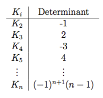
$ K_n $ has the eigenvalues $ -1, -1, ..., -1 $ where $ -1 $ has multiplicity $ n - 1 $. The determinants of $ K_n $ are as follows:
Eigenvalue and Graph Diameter Theorem:
If the diameter of $ G $ is $ d $, then the cardinality of the spectrum of $ A $ are related by: $$ \big| \sigma(A) \big| \geq d + 1 $$
Bipartite Graph Theorem:
The graph $ G $ is bipartite if and only if the collection of eigenvalues of $ G $ is symmetric about 0. $ \lambda_n = - \lambda_1 $ for any bipartite graph.
Graph complements and Eigenvalues Theorem:
Let $ G $ be a graph of order $ n $ which is regular and of degree $ k $. Let $ \sigma(G) = \lambda_n, \lambda_{n-1}, ..., \lambda_1 $. Let $ \lambda_1 = k $. Then the eigenvalues of $ \bar{G} $ are $ n-1-k, -1 - \lambda_n, ..., -1 - \lambda_n$.
Chromatic Number and Largest Eigenvalue Theorem:
$ \chi(G) \leq \lambda_1(G) + 1 $

There are many more theorems - and they reach deeply into several branches of mathematics. My interest in this is that I can find useful information about structures that may be represented as graphs. It would be cool to have some code for generating adjacency matrices and the eigenstuff for any arbitrary graph. If this can be done for an arbitrary case, it will work for any particular case I may wish to examine.

To this end, I wrote some Mathematica code. The program generates a pseudo random $ n \times n $ adjacency matrix of either zeros or ones. It then discards nonsymmetric entries by grabbing the upper triangular matrix and adding it to its own transpose. The diagonal entries (in the irreflexive case) should be zero so it subtracts twice the value of the diagonals in the original matrix from the now symmetric matrix.

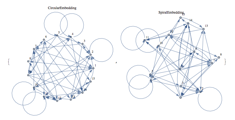
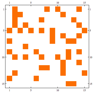
I have written variations of this to produce reflexive graphs, directed graphs, and combinations of these. I used Mathematica here because it has powerful graph rendering capability and will draw 'circular' and 'spiral' embeddings as well as matrix plots with a single command. Mathematica then calculates the eigenvalues of the generated graph using built-in functions.

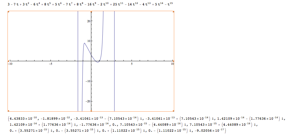
To check the calculations, the program generates the characteristic polynomial and plugs eigenvalues into it. The result should be close to zero for each eigenvalue. It also plots the characteristic polynomial so it is easy to see the eigenvalues quickly.

Some screen captures of results (Directed / Reflexive case with a randomly generated set of edges for 25 vertices):
Graph Embeddings Matrix Plot Characteristic Polynomial

Mathematica Code:
I normally comment in code I write but these are completely uncommented. If you have a question about the Mathematica files contact me and I'll try to answer your question.