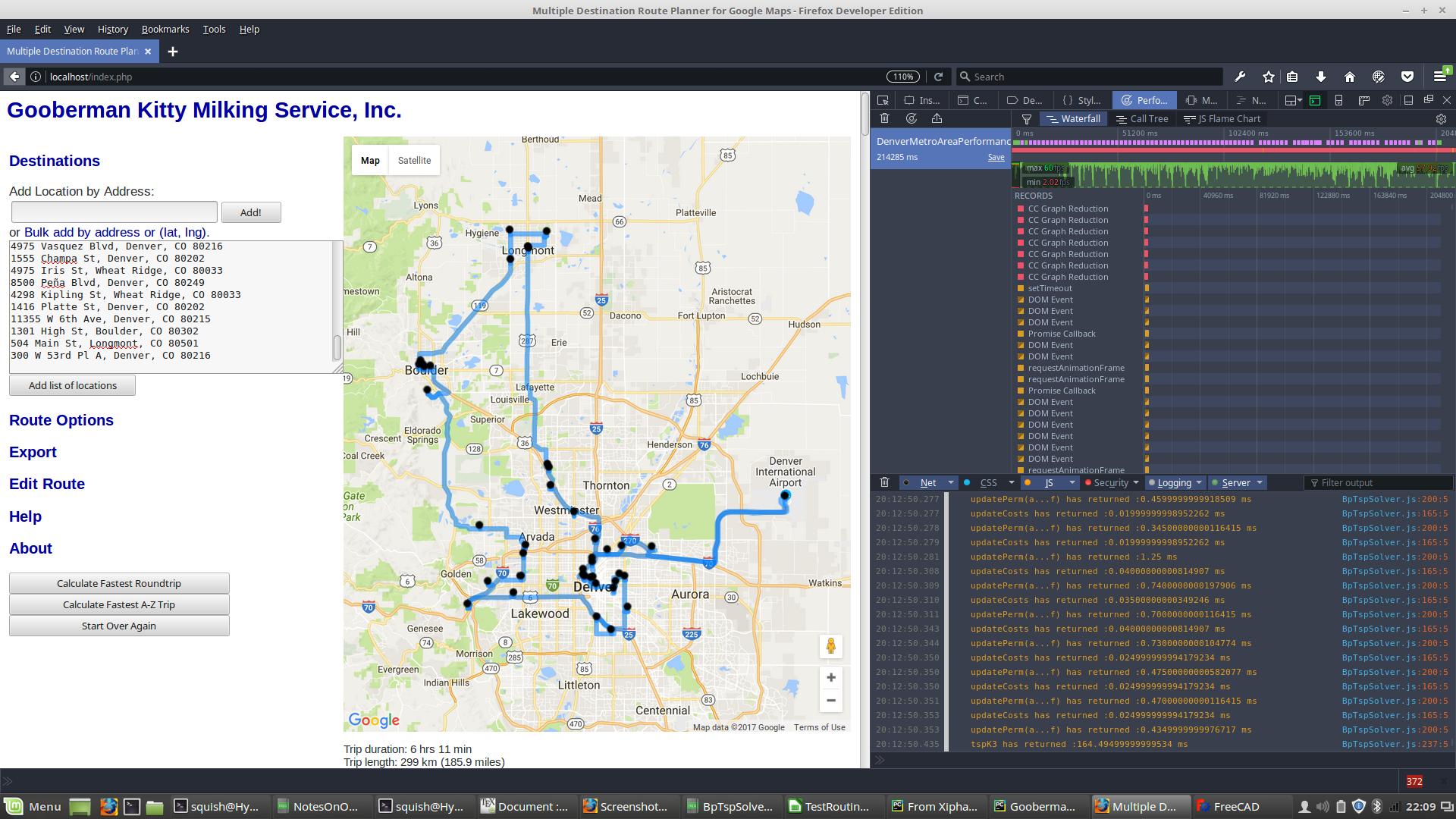
The main JavaScript algorithm BpTspSolver.js has been modified to utilize the performance.now() method which may be used to time functions in milliseconds as they are executed. The stated accuracy is ± 5 microseconds. The output is posted to the JavaScript console log.
var t0 = performance.now();
do_something();
console.log("function do_something has returned :" + (performance.now() - t0) + " ms");
The console log can be analyzed to see individual components of the algorithm code and server POST messages execute with an accurate timer. Firefox Developer Edition has a useful set of plotting functions to visualize these logs. The console log was then copied into a spreadsheet and analyzed with Python.
- Boulder addresses
- Boulder and Longmont addresses
- Boulder, Longmont, and Denver addresses
3(5) + 3(10) + 3(15) + ... + 3(45) + 2(50) = 775
results in over 20,000 POST calls to the Google Maps API. This exceeds the limit set in a 24 hour period:
"You have exceeded your daily request quota for this API. We recommend registering for a key at the
Google Developers Console: https://console.developers.google.com/apis/credentials?project=_
For more information on authentication and Google Maps Javascript API services please see:
https://developers.google.com/maps/documentation/javascript/get-api-key"

Whoops!
Whatever missing tests have since been run. Analysis of these follows.
When our site goes live we will need to purchase API executions. But that is what we call a high quality problem because we will have paying customers if we exceed 20,000 API calls!
The server execution is broken (loosely) into the following stages:
- Paint Initialization: These are the steps utilized to draw the initial webpage before user input.
- Initial geo-location POST calls to Google: These are the geo-location calls to find the addresses put in by a user. This process was not timed because user input is still required and the TSP algorithm is not yet called.
- Initialization: These are the steps taken by the server when "Find Optimal Route" is initiated by the user. Typical calls look like this:
The first entry is a recurring error due to depreciation of a JavaScript method.12:44:46.209 Use of getAttributeNode() is deprecated. Use getAttribute() instead. jquery.min.js:2:29939 12:44:46.217 GET http://maps.googleapis.com/maps-api-v3/api/js/27/12/geometry.js [HTTP/1.1 200 OK 0ms] 12:44:46.219 GET http://maps.googleapis.com/maps-api-v3/api/js/27/12/directions.js [HTTP/1.1 200 OK 0ms] - POST calls to the Google Maps API: These POST calls get address information that is used by the TSP algorithm. These calls take up the largest part of the execution time. They look like this:
- Server BpTspSolver.js execution: Most of the hard work is done here. This is where the algorithm actually determines the optimal route. The method calls should look familiar.
- Post-algorithm paint of determined route: Once the algorithm is done crunching to find an optimal solution the screen has to be redrawn.
12:44:46.258 GET  http://maps.googleapis.com/maps/api/js/DirectionsService.Route [HTTP/1.1 200 OK 0ms]
12:44:46.285 GET  http://maps.googleapis.com/maps/api/js/DirectionsService.Route [HTTP/1.1 200 OK 0ms]
12:44:46.326 GET  http://maps.googleapis.com/maps/api/js/DirectionsService.Route [HTTP/1.1 200 OK 0ms]
12:44:46.347 GET  http://maps.googleapis.com/maps/api/js/DirectionsService.Route [HTTP/1.1 200 OK 0ms]
12:44:46.370 GET  http://maps.googleapis.com/maps/api/js/DirectionsService.Route [HTTP/1.1 200 OK 0ms]
12:44:46.372 GET  http://maps.googleapis.com/maps/gen_204 [HTTP/1.1 204 No Content 50ms]
12:44:46.404 GET  http://maps.googleapis.com/maps/api/js/DirectionsService.Route [HTTP/1.1 200 OK 0ms]
12:44:46.432 GET  http://maps.googleapis.com/maps/api/js/DirectionsService.Route [HTTP/1.1 200 OK 0ms]
12:44:46.468 GET  http://maps.googleapis.com/maps/api/js/DirectionsService.Route [HTTP/1.1 200 OK 740ms]
12:44:47.236 GET  http://maps.googleapis.com/maps/api/js/DirectionsService.Route [HTTP/1.1 200 OK 790ms]
12:44:48.049 GET  http://maps.googleapis.com/maps/api/js/DirectionsService.Route [HTTP/1.1 200 OK 1000ms]
12:44:48.049 GET  http://maps.googleapis.com/maps/gen_204 [HTTP/1.1 204 No Content 38ms]
12:44:49.075 GET  http://maps.googleapis.com/maps/api/js/DirectionsService.Route [HTTP/1.1 200 OK 586ms]
12:50:54.454 costPerm(a...f) has returned :1.125 ms  BpTspSolver.js:145:5
12:50:54.455 cost(a,b) has returned :0 ms  BpTspSolver.js:123:7
12:50:54.456 costPerm(a...f) has returned :1.1300000000046566 ms  BpTspSolver.js:145:5
12:50:54.456 cost(a,b) has returned :0 ms  BpTspSolver.js:123:7
12:50:54.457 costPerm(a...f) has returned :1.099999999976717 ms  BpTspSolver.js:145:5
12:50:54.457 cost(a,b) has returned :0 ms  BpTspSolver.js:123:7
12:50:54.458 cost(a,b) has returned :0.005000000004656613 ms  BpTspSolver.js:123:7
12:50:54.459 costPerm(a...f) has returned :1.2449999999953434 ms  BpTspSolver.js:145:5
12:50:54.459 cost(a,b) has returned :0 ms  BpTspSolver.js:123:7
12:50:54.460 costPerm(a...f) has returned :1.1050000000395812 ms  BpTspSolver.js:145:5
12:50:54.460 cost(a,b) has returned :0 ms  BpTspSolver.js:123:7
12:50:54.461 cost(a,b) has returned :0.005000000004656613 ms  BpTspSolver.js:123:7
12:50:54.461 cost(a,b) has returned :0 ms  BpTspSolver.js:123:7
12:50:54.461 costPerm(a...f) has returned :1.095000000030268 ms  BpTspSolver.js:145:5
12:50:54.464 tspK3 has returned :189202.99 ms  BpTspSolver.js:239:5
12:50:54.691 prepareSolution has returned :225.45999999996275 ms  BpTspSolver.js:805:5
12:50:54.691 doTsp has returned :189495.93 ms  BpTspSolver.js:764:5
12:50:54.692 readyTsp has returned :189499.135 ms  BpTspSolver.js:736:5
12:50:57.334 GET  http://localhost/blackdot.png [HTTP/1.1 304 Not Modified 0ms]
12:50:59.670 GET  http://maps.googleapis.com/maps-api-v3/api/js/27/12/infowindow.js [HTTP/1.1 200 OK 0ms]
12:50:59.681 GET  http://maps.googleapis.com/maps-api-v3/api/js/27/12/poly.js [HTTP/1.1 200 OK 0ms]
12:51:00.043 GET  http://maps.gstatic.com/mapfiles/undo_poly.png [HTTP/1.1 304 Not Modified 30ms]
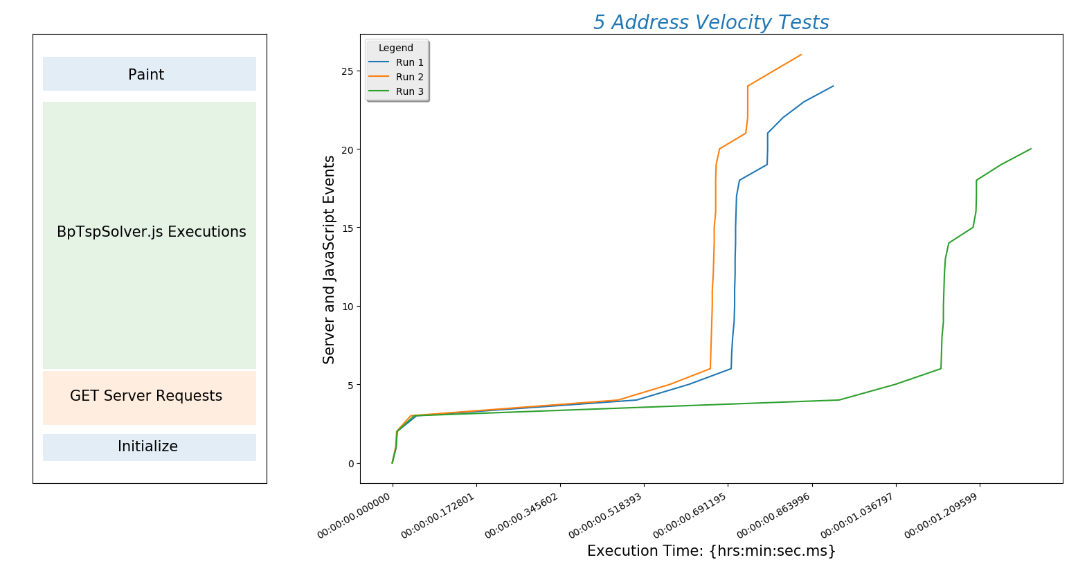
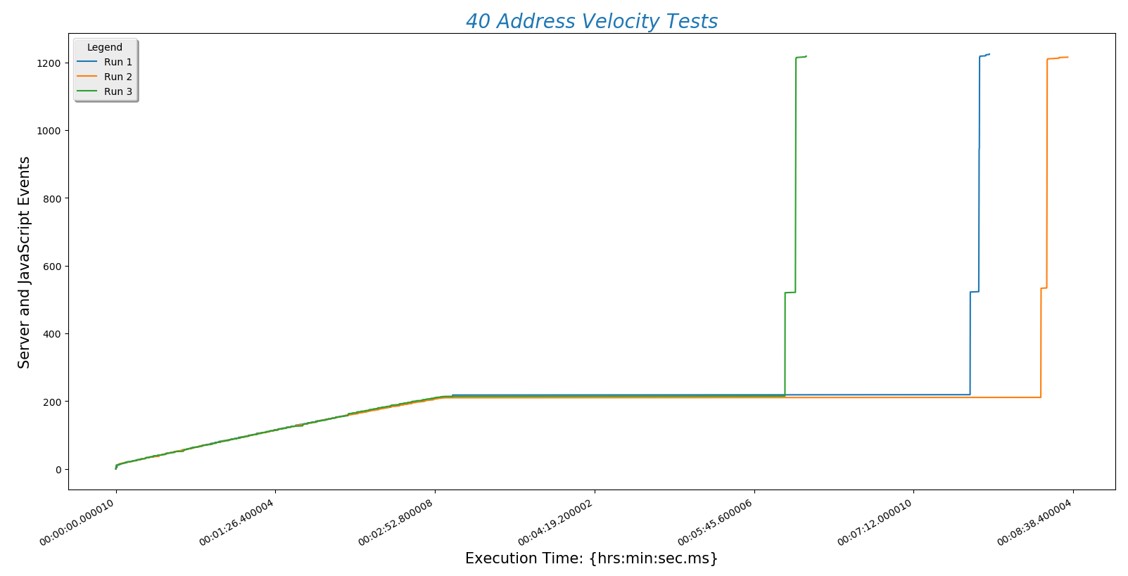
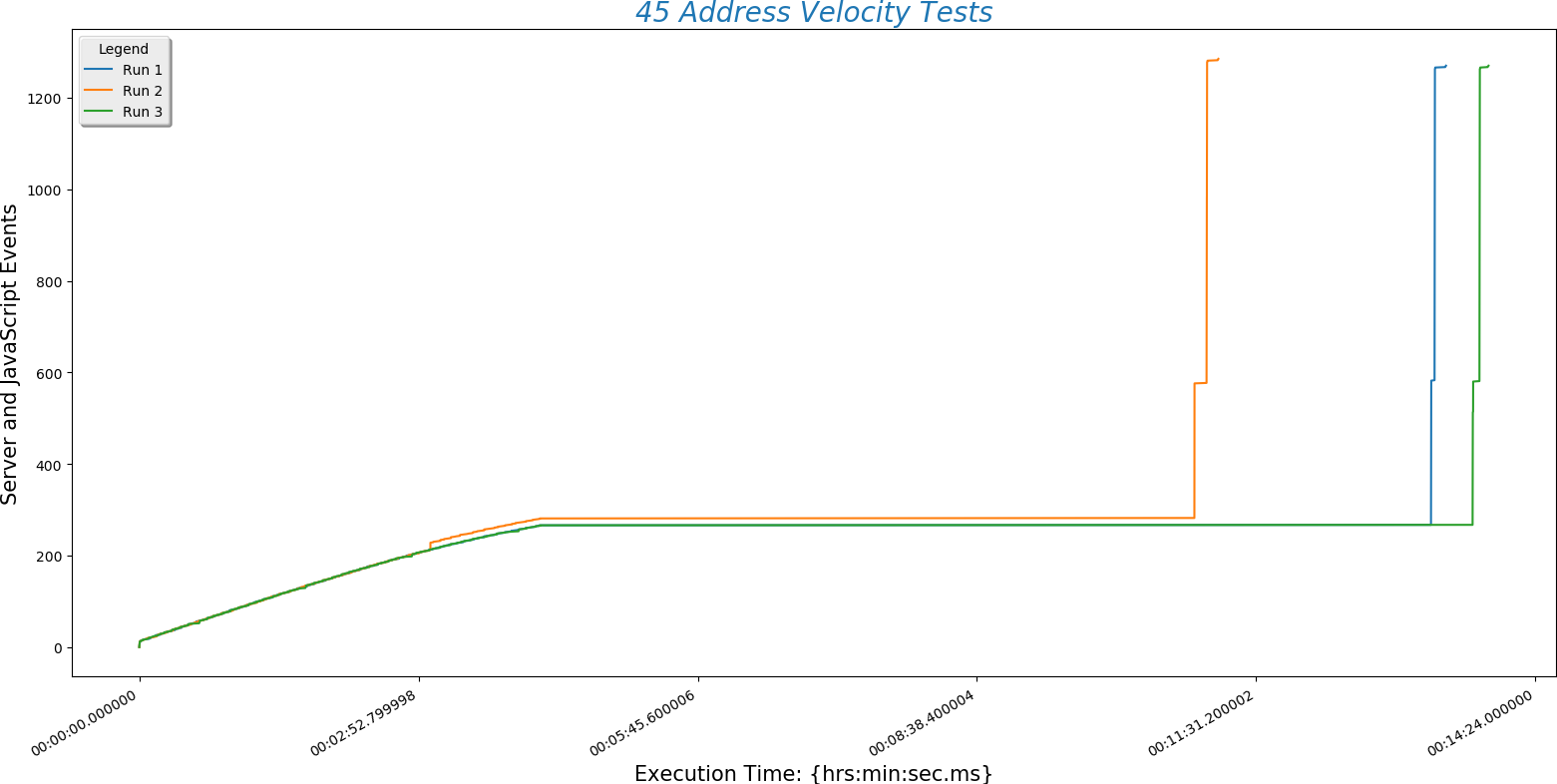
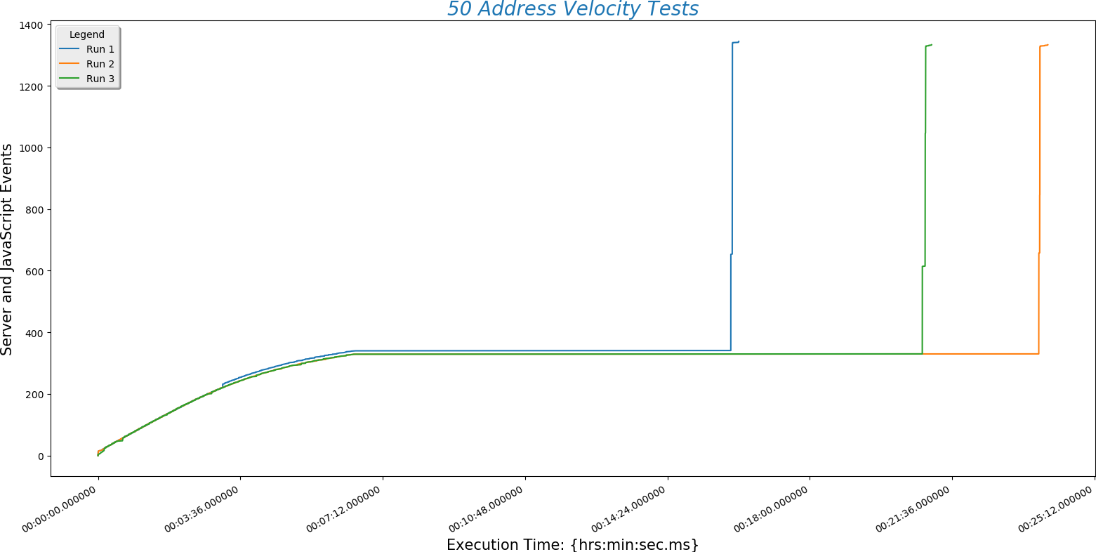
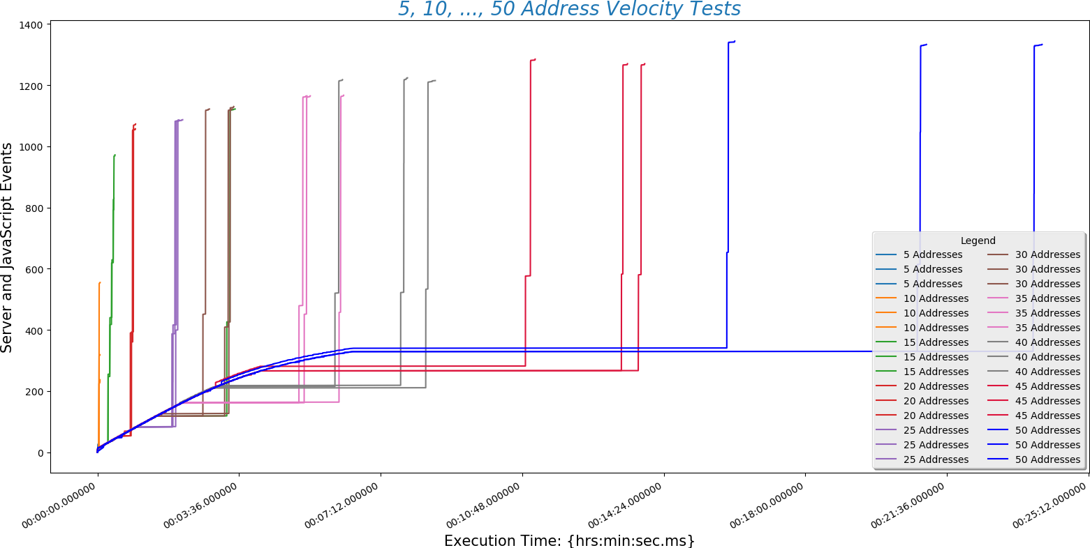
The plot(above) describes the behavior of all subsequent plots.
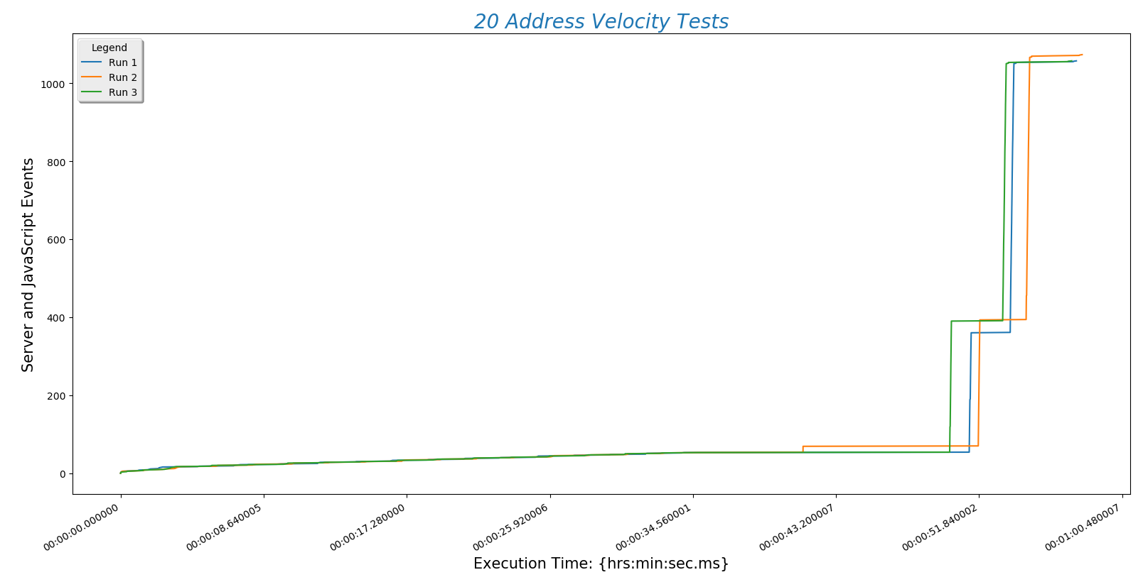
The x-axis is time and \(y\)-axis is work being done by the site. The steeper the line the better! A steep line means that a lot of work is being done quickly. The nearly horizontal lines toward the bottom of the plot are the slowest part of the algorithm. This is where the site is sending and receiving data from Google. This is also the part of the process we have the least control over but we can probably find a way to make this part of the process faster. We may, for example, decide to cache these responses if a user is repeatedly calling for the same address. The most important thing to learn here is that initially internet connection speed will be more important than server processor speed. Of course the processor will start to matter when multiple users are on the site and we add a lot of user functionality.
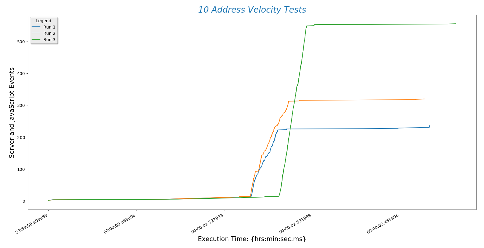
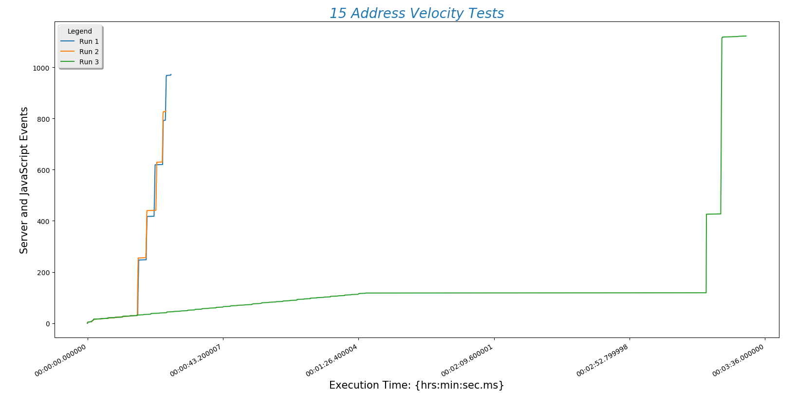
The following plots are tests run with 10, 15, 20, 30, and 40 addresses each. I will run tests with hundreds of addresses as soon as my API key isn't maxed out. 10 addresses:
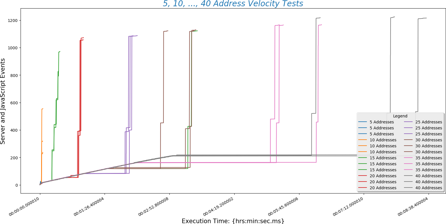
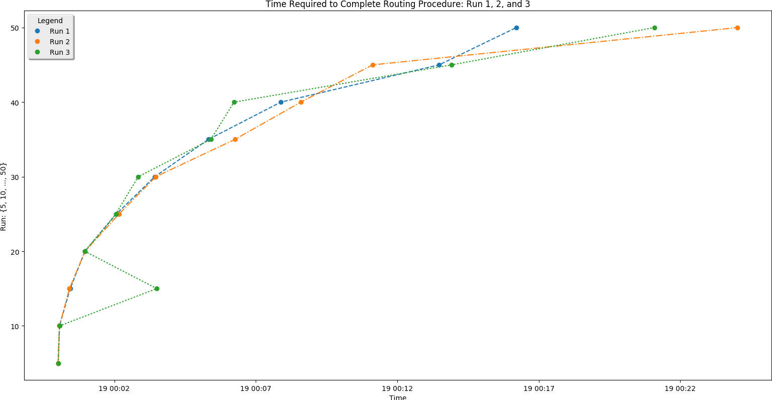
This is a plot comparing the number of addresses (\(y\)-axis) against the time a run took to complete ($x$-axis)
This is a different way at looking at the same data. Here the number of addresses entered (\(x\)-axis) is plotted against normalized time (\(y\)-axis).
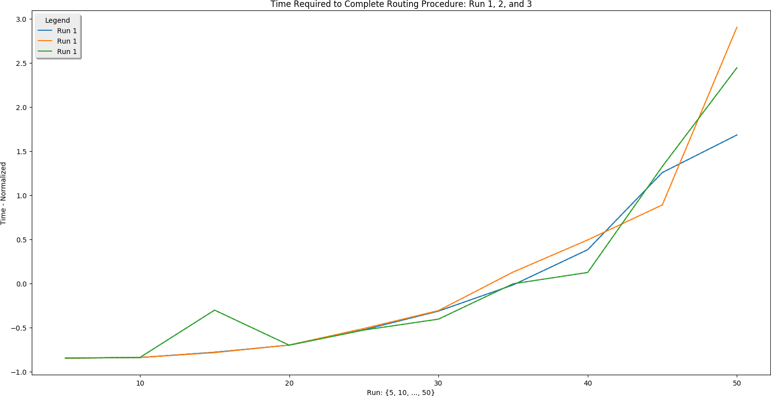
There are a few conclusions we may draw from this information:
- Server POST time is reliably the slowest part of finding a route. This is determined by the speed of the internet connection. Choosing a hosting service with fast throughput will be essential.
- The BpTspSolver.js code is probably fast enough, without modification, to serve a future site. That means we can use existing code without doing more work like writing compiled C to increase site speed.
- Recall that there are three address sets. Set 1 (always plotted as run 1) is only local Boulder addresses. Set 3 (always plotted as run 3) contains Denver metro area addresses including Longmont and Boulder. This means that the third set is of higher complexity. However, this does not increase the time needed for the site to process the addresses. That means that input complexity is not a significant factor in how long the site takes to return a route.
Python Code
This is some of the Python code used to perform the `Velocity Tests' analysis. The JavaScript Console data has to be reformatted:
# Routing Data Reformatting Tool
# Eric Johnson -- eric@focusNumeric.net

import numpy as np
import pandas as pd

# NOTE:  The blank rows printed to the end of this file are causing problems!  Fix it!

inputFilename = 'RoutingTestRuns.xlsx'
destinationFilename = 'RoutingTestRunsReformatted.xlsx'
# Required -- how many sheets are there?
numSheets = 8

# Initialize excel writer
writer = pd.ExcelWriter(destinationFilename)

for sheetIndex in range(0,numSheets):
    thisSheet = pd.read_excel(inputFilename, sheetname=sheetIndex)
    # pulls sheets.  Sheet 9 only has two runs.
    thisRunData1 = pd.Series(thisSheet['Set1'],dtype=str)
    thisRunData2 = pd.Series(thisSheet['Set2'],dtype=str)
    thisRunData3 = pd.Series(thisSheet['Set3'],dtype=str)
    # Perform the remainder of the processing on run 1
    for index in range(0, len(thisRunData1)):
        thisLine = thisRunData1[index]
        if not thisLine.startswith('h'):
            #print("Does not start with h")
            thisRunData1[index] = thisRunData1[index]
            # print(set1_5[index])
        if thisLine.startswith('h'):
            #print("starts with h")
            thisRunData1[index - 1] = thisRunData1[index - 1] + " " + thisRunData1[index]
            thisRunData1[index] = 'nan'
            # print(set1_5[index-1])
    # Now pull the lines that is not 'nan'
    thisRunData1 = thisRunData1.replace('nan', np.nan)
    thisRunData1 = thisRunData1.dropna()
    print(thisRunData1)
    thisRunData1 = pd.DataFrame(thisRunData1)
    sheet = str(5+5*sheetIndex) + str(" Run 1")
    thisRunData1.to_excel(writer, sheet_name=sheet)
    # Perform the remainder of the processing on run 2
    for index in range(0, len(thisRunData2)):
        thisLine = thisRunData2[index]
        if not thisLine.startswith('h'):
            # print("Does not start with h")
            thisRunData2[index] = thisRunData2[index]
            # print(set1_5[index])
        if thisLine.startswith('h'):
            # print("starts with h")
            thisRunData2[index - 1] = thisRunData2[index - 1] + " " + thisRunData2[index]
            thisRunData2[index] = 'nan'
            # print(set1_5[index-1])
    # Now pull the lines that is not 'nan'
    thisRunData2 = thisRunData2.replace('nan', np.nan)
    thisRunData2 = thisRunData2.dropna()
    print(thisRunData2)
    thisRunData2 = pd.DataFrame(thisRunData2)
    sheet = str(5+5*sheetIndex) + str(" Run 2")
    thisRunData2.to_excel(writer, sheet_name=sheet)
    # Perform the remainder of the processing on run 3
    for index in range(0, len(thisRunData3)):
        thisLine = thisRunData3[index]
        if not thisLine.startswith('h'):
            # print("Does not start with h")
            thisRunData3[index] = thisRunData3[index]
            # print(set1_5[index])
        if thisLine.startswith('h'):
            # print("starts with h")
            thisRunData3[index - 1] = thisRunData3[index - 1] + " " + thisRunData3[index]
            thisRunData3[index] = 'nan'
            # print(set1_5[index-1])
    # Now pull the lines that is not 'nan'
    thisRunData3 = thisRunData3.replace('nan', np.nan)
    thisRunData3 = thisRunData3.dropna()
    print(thisRunData3)
    thisRunData3 = pd.DataFrame(thisRunData3)
    sheet = str(5+5*sheetIndex) + str(" Run 3")
    thisRunData3.to_excel(writer, sheet_name=sheet)

writer.save()

\end{verbatim}
\begin{center}
\textbf{This is the 5 address plotting code:}
\end{center}
\begin{verbatim}
# Routing Performance Data Plotting
# Eric Johnson -- eric@focusNumeric.net

import pandas as pd
import matplotlib.pyplot as plt
from datetime import datetime
import matplotlib.dates as mdates
import matplotlib.dates as dates
from matplotlib import gridspec


inputFilename = 'RoutingTestRunsReformatted.xlsx'
destinationFilename = ''

# read from file
dataSheet = pd.read_excel(inputFilename, sheetname=0)
runData1 = pd.Series(dataSheet['Set1'], dtype=str)
runData1 = runData1.sort_values()
dataSheet = pd.read_excel(inputFilename, sheetname=1)
runData2 = pd.Series(dataSheet['Set2'], dtype=str)
runData2 = runData2.sort_values()
dataSheet = pd.read_excel(inputFilename, sheetname=2)
runData3 = pd.Series(dataSheet['Set3'], dtype=str)
runData3 = runData3.sort_values()

# Normalize all timestamp info - keep track in timeList()

# Time format - required for datetime
FMT = '%H:%M:%S.%f'
# For data part 1
# Time list - to keep track of timeElapsed
timeList1 = list()
# Data definitions
firstLine1 = runData1[0]
firstLine1 = list(firstLine1.split(" "))
timeZero1 = firstLine1[0]
# Normalize time
for thisRow1 in runData1:
    thisList1 = list(thisRow1.split(" "))
    timeElapsed1 = str(datetime.strptime(thisList1[0], FMT) - datetime.strptime(timeZero1, FMT))
    thisList1[0] = timeElapsed1
    thisRow1 = thisList1
    timeList1.append(timeElapsed1)
# Add milliseconds to first element
timeList1[0] += ".000000"

print(timeList1)

events1 = range(0,len(timeList1))
print(len(events1))
print(len(timeList1))

# For data part 2
# Time list - to keep track of timeElapsed
timeList2 = list()
# Data definitions
firstLine2 = runData2[0]
firstLine2 = list(firstLine2.split(" "))
timeZero2 = firstLine2[0]
# Normalize time
for thisRow2 in runData2:
    thisList2 = list(thisRow2.split(" "))
    timeElapsed2 = str(datetime.strptime(thisList2[0], FMT) - datetime.strptime(timeZero2, FMT))
    thisList2[0] = timeElapsed2
    thisRow2 = thisList2
    timeList2.append(timeElapsed2)
# Add milliseconds to first element
timeList2[0] += ".000000"

print(timeList2)

events2 = range(0,len(timeList2))
print(len(events2))
print(len(timeList2))

# For data part 3
# Time list - to keep track of timeElapsed
timeList3 = list()
# Data definitions
firstLine3 = runData3[0]
firstLine3 = list(firstLine3.split(" "))
timeZero3 = firstLine3[0]
# Normalize time
for thisRow3 in runData3:
    thisList3 = list(thisRow3.split(" "))
    timeElapsed3 = str(datetime.strptime(thisList3[0], FMT) - datetime.strptime(timeZero3, FMT))
    thisList3[0] = timeElapsed3
    thisRow3 = thisList3
    timeList3.append(timeElapsed3)
# Add milliseconds to first element
timeList3[0] += ".000000"

print(timeList3)

events3 = range(0,len(timeList3))
print(len(events3))
print(len(timeList3))

# Now plot
x1 = dates.datestr2num(timeList1)
x2 = dates.datestr2num(timeList2)
x3 = dates.datestr2num(timeList3)
y1 = events1
y2 = events2
y3 = events3
gs = gridspec.GridSpec(1, 2, width_ratios=[1, 3])
ax1 = plt.subplot(gs[0])
ax1.axis('on')
ax1.axes.get_xaxis().set_ticks([])
ax1.axes.get_yaxis().set_ticks([])
ax1.axvspan(xmin=0, xmax=.2, ymin=.05, ymax=.11, facecolor='#1f77b4', alpha=0.125)
ax1.text(.07, .073, 'Initialize', fontsize=15)
ax1.axvspan(xmin=0, xmax=.2, ymin=.13, ymax=.25, facecolor='#ff7f0e', alpha=0.125)
ax1.text(.025, .185, 'GET Server Requests', fontsize=15)
ax1.axvspan(xmin=0, xmax=.2, ymin=.255, ymax=.85, facecolor='#2ca02c', alpha=0.125)
ax1.text(.013, .55, 'BpTspSolver.js Executions', fontsize=15)
ax1.axvspan(xmin=0, xmax=.2, ymin=.875, ymax=.95, facecolor='#1f77b4', alpha=0.125)
ax1.text(.08, .9, 'Paint', fontsize=15)

txt = ax1.text(0.5, 0.5, "test", size=30, ha="center", color="w")
ax2 = plt.subplot(gs[1])
plt.gca().xaxis.set_major_formatter(mdates.DateFormatter('%H:%M:%S.%f'))
plt.plot(x1,y1,label="Run 1", color='#1f77b4')
plt.plot(x2,y2,label="Run 2", color='#ff7f0e')
plt.plot(x3,y3,label="Run 3", color='#2ca02c')
plt.title("5 Address Velocity Tests", fontsize=20, color='#1f77b4', fontstyle='oblique')
plt.xlabel("Execution Time: {hrs:min:sec.ms}", fontsize=15)
plt.ylabel("Server and JavaScript Events", fontsize=15)
plt.legend(loc="upper left", bbox_to_anchor=[0, 1], ncol=1, shadow=True, title="Legend", fancybox=True)
plt.gcf().autofmt_xdate()
plt.show()