Polynomial Best Fit with Matlab

Polynomial best fit with R

A least-squares polynomial fit is a useful technique for finding a function that roughly approximates data. Consider the following plot as an example:

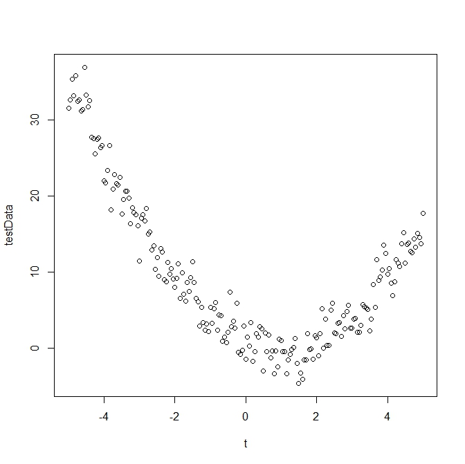
The data looks similar to a quadratic function - but with lots of noise. To approximate data values, we do not want a function that goes through every data point. To do so would produce a uselessly long polynomial with extremely high order. If we had 50 data points, for instance, we might have to have a 50+ degree polynomial which would be impractical and silly. And then what happens when we add a new data point? We would have to recalculate our 'approximation' right from the beginning. Instead, we can simply approximate this data with a quadratic function and get reasonably close. Most of the time 'reasonably close' will be good enough.

I wanted to write some Matlab code to produce a least-squares polynomial of arbitrary order for overdetermined data (more than full-rank). The first two sets of Matlab code are for creating second and third-degree polynomial least-squares functions. The last part is code to produce a least-squares polynomial of arbitrary order. In addition to the Matlab code, I also had to produce some test data sets. R code to produce those sets (with error added artificially) is also here.

Here is a general mathematical explanation of how a least-squares problem is solved. Matlab and R have built-in functions for performing least-squares polynomial curve-fitting, but I'd much rather write something of my own!

Suppose we have an system $ Ax = b $ where $A \in \mathbb{R}^{n \times m} $, $ b \in \mathbb{R}^n $, where $ n > m $. This makes the system $ Ax = b $ overdetermined, and makes $ A $ non-square. We want to find some unknown $ x $ that minimizes the 2-norm residual:

$$ \Vert r \Vert_2 = \Vert b - Ax \Vert_2 $$

To solve this we will take advantage of $ QR $ decomposition and minimize the residual $ s = Q^T b - Q^T A x $ of the transformed system

$$ Q^T A x = Q^T b $$

The matrix $ Q $ is orthogonal. That matters to us here because orthogonal matrices do not change matrix norms. In other words, the 2-norm of the residual $ r $ is the same as the residual $ s $ of the transformed system. Let $ c = Q^T b $, and do the following:

Recall that with $ QR $ decomposition, we have $Q^T Q = I $, and so $ A = QR $, and $ R = Q^T A $. Use Matlab to perform the actual decomposition and find $ R $.
Solve $ Q c = b $ for $ c $.
Find $ Rx = c $ by back substitution to find $ x $. The vector $ x $ has all of the coefficients of the least-squares polynomial that best approximates the data.

Steps (1), (2), and (3) are performed with the following Matlab code. The matrix $ A $ is built earlier in the program (see below).

b = b';          % This is the data. We need it to be a column vector so perform a transpose.
[Q, R] = qr(A);  % Use the QR decomposition function built-in to Matlab.
c = Q'*b;        % Let c = Q^T b
x = R\c;         % solve for x

The construction of the matrix $ A $ requires that we pick a polynomial basis that depends on our desired polynomial order. The standard bases for polynomials are just \begin{align*} \phi_1(z) + \phi_2(z) &= 1 + z \\ \phi_1(z) + \phi_2(z) + \phi_3(z) &= 1 + z + z^2 \\ \phi_1(z) + \phi_2(z) + \phi_3(z) + \phi_4(z) &= 1 + z + z^2 + z^3 \\ &\vdots \\ \phi_1(z) + \phi_2(z) + ... + \phi_{n-1}(z) &= 1 + z + ... + z^{n-1} + z^n \end{align*}

We let the $ i^{\text{th}} $ independent variable be $ t_i $ and construct $ A $: \begin{align} A = \begin{pmatrix} \phi_1(t_1) & \phi_2(t_1) & \cdots & \phi_{n-1}(t_1) \\ \phi_1(t_2) & \phi_2(t_2) & \cdots & \phi_{n-1}(t_2) \\ \vdots & \vdots & \ddots & \vdots \\ \phi_1(t_n) & \phi_2(t_n) & \cdots & \phi_{n-1}(t_n) \\ \end{pmatrix} \end{align}

This is accomplished in Matlab (for the 2nd degree polynomial case) with the following:

A(1:dataSize,1) = 1;
A(1:dataSize,2) = t(1,1:dataSize);
A(1:dataSize,3) = (t(1,1:dataSize)).^2;

Here is the full Matlab code to find a second degree polynomial fit:

function LeastSquaresDegree2(t,b)
% usage:  t is independent variable vector, b is function data 
% i.e., b = f(t)
% This works only for second degree polynomial 
% Try t = -5:0.05:5 with SecondDegreeTestData.dat
%
dataSize = length(b);
A = zeros(dataSize,3);
%
% Given basis phi(z) = 1 + z + z^2
A(1:dataSize,1) = 1;
A(1:dataSize,2) = t(1,1:dataSize);
A(1:dataSize,3) = (t(1,1:dataSize)).^2;
% 
b = b';
[Q,R] = qr(A);
c = Q'*b;
x = R\c;
%
plot(t(1:dataSize),b(1:dataSize),'r*', t(1:dataSize), x(1,1) + x(2,1)*t(1:dataSize) + x(3,1)*(t(1:dataSize)).^2,'k')
title('Data plotted with 2nd Degree Least Squares Polynomial', 'FontWeight', 'bold', 'Color', 'b', 'FontSize', 14)
xlabel('independent variable t', 'FontWeight', 'bold', 'FontSize', 12)
ylabel('function values f(t)', 'FontWeight', 'bold', 'FontSize', 12)
legend('Input Data', 'Second Degree Polynomial')
axis tight
%
% For debugging:
% length(t);
% length(b);
%
% Check
Soln = A\b
Resid = Soln - x
%
% Code by Eric Johnson -- Focus | Numeric
end

For a third degree polynomial, we just have to construct a bigger matrix.

A(1:dataSize,1) = 1;
A(1:dataSize,2) = t(1,1:dataSize);
A(1:dataSize,3) = (t(1,1:dataSize)).^2;
A(1:dataSize,4) = (t(1,1:dataSize)).^3;

Calculating a polynomial of arbitrary order is a little more complicated. We pass the desired polynomial order to Matlab as an argument. The matrix $ A $ has to be created based on the desired polynomial order. And the vector that is used to plot out the least-squares polynomial can be written dynamically using a simple loop.

Here's the loop for constructing the matrix $ A $:

% Given basis phi(t) = 1 + t + t^2 + ... + t^n
% Initialize A
A(1:dataSize,1) = 1;
% Fill in the rest of A
for i = 1:1:n
    A(1:dataSize,i+1) = (t(1,1:dataSize)).^(i);
end

And here is the loop that allows us to graph the interpolated function. We have to make an appropriate change in the plotting command to plot 'xPlot.'

% initialize xPlot with the right starting value
xPlot = x(1,1);
% create the rest of the entries
for i = 1:1:n
    xPlot = xPlot + x(i+1,1)*(t(1:dataSize)).^i;
end

Some numerical experiments utilizing this technique...

Here is a plot of the function output of LeastSquaresDegree2(t2,SecondDegreeTestData) where t2 = -5:0.05:5, and SecondDegreeTestData was imported from the *dat file (download below).

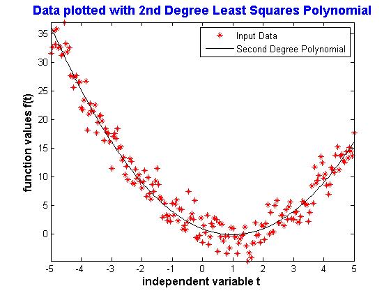
The coefficients output are: \begin{align} \phi_1(t) &= 1.0097 \\ \phi_2(t) &= -2.0223 \\ \phi_3(t) &= 0.9527 \end{align}
Which makes the second-degree polynomial that best fits the data \begin{align} \phi(t) = 0.9527 t^2 - 2.0223 t + 1.0097 \end{align} which is pretty good because I started with the polynomial \begin{align} p(t) = t^2 - 2 t + 1. \end{align}

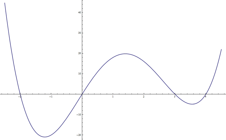
Here is a plot of the function output of LeastSquaresDegree3(t3,ThirdDegreeTestData) where t3 = 1:0.025:9, and ThirdDegreeTestData was imported from the *.dat file (download below).

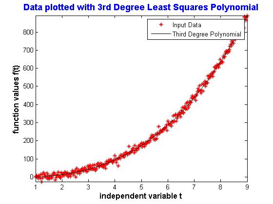
The coefficients output are: \begin{align} \phi_1(t) &= 1.0372 \\ \phi_2(t) &= 1.3443 \\ \phi_3(t) &= 3.4257 \\ \phi_4(t) &= -6.8168 \end{align}

Here is a plot of the function output of LeastSquaresDegreeN(t9,NinthDegreeTestData,9) where t9 = -2.6:0.005:1.8, and NinthDegreeTestData was imported from the *.dat file (download below).

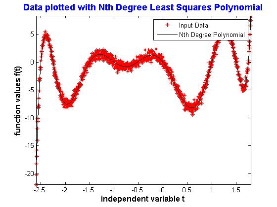
The coefficients output are: \begin{align} \phi_1(t) &= 1.0069 \\ \phi_2(t) &= 3.5363 \\ \phi_3(t) &= -4.4279 \\ \phi_4(t) &= -22.7728 \\ \phi_5(t) &= 0.9491 \\ \phi_6(t) &= 44.5857 \\ \phi_7(t) &= 13.8822 \\ \phi_8(t) &= -25.2969 \\ \phi_9(t) &= -11.3785 \\ \phi_{10}(t) &= 0.0237 \end{align}
This is also very good since I started with this polynomial:

Ninth-Degree Polynomial

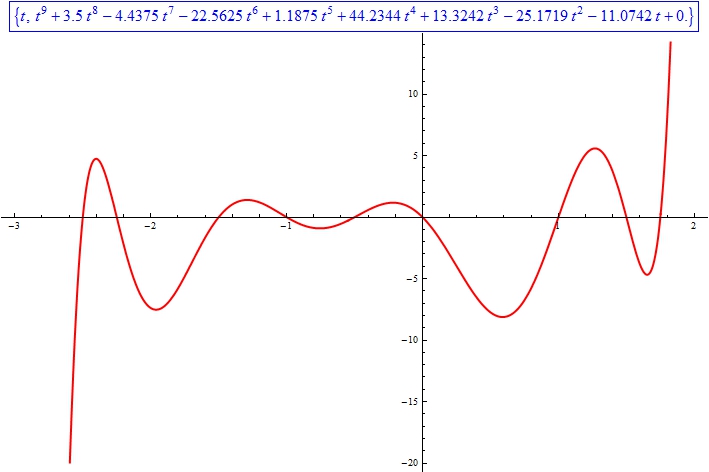
In any case I am confident that the code works!

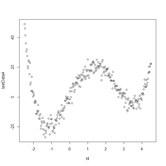
The data sets were created in R using this method:

Create an evenly spaced vector by typing something like:
```
t4 <- seq(-2.5, 4.5, 0.025)
```
Create points that follow your chosen polynomial by typing something like:
```
y4 <- (t4)^4 - 5*(t^4)^3 -2*(t4)^2 + 24*(t4)
```
Create a normally distributed amount of noise by typing something like:
```
err4 <- rnorm(281, mean = 0, sd = 3)
```
Now just add 'y4' and 'err4'. To create the forth-degree polynomial data I actually used this:
```
testData4 <- y4 + 4*err4
```
Ta da!

The last step transforms the data into something fuzzier and more interesting to work with... Forth-Degree Polynomial

$ \ \ \to \ \ $ Forth-Degree Polynomial with Noise

An additional note about the Matlab code:

Matlab requires the the function arguments "t" and "b" be vectors of equal length. It will fail if you don't perform this step correctly! There are comments in each of the Matlab files that should help. If you can't make them work, email me and I'll try to clarify.

I have not tested this code on any data that will produce a less than full rank matrix $ A $.

Links to Matlab code:
Matlab Code for finding second degree polynomial
Matlab Code for finding third degree polynomial
Matlab Code for finding any arbitrary degree polynomial
Depending on your browser you may have to 'save as.'

Links to the data sets (with uniformly distributed noise added). You will have to import the data into Matlab.
Second degree polynomial data with added noise Try t = -5:0.05:5
Third degree polynomial data with added noise Try t = 1:0.025:9 {This looks quadratic - but is actually third degree!}
Forth degree polynomial data with added noise Try t = -2.5:0.025:4.5
Ninth degree polynomial data with added noise Try t = -2.6:0.005:1.8
Depending on your browser you may have to 'save as.'

Some places to find out more:

Fundamentals of Matrix Computations by David Watkins. This is a beautifully written book by one of my favorite professors from WSU. I highly recommend it!
Least Squares Polynomial Fitting from Mathworld.
Least Squares Polynomial Fitting using R instead of Matlab (by me).